
2013 has been an amazing year for the RECON project. We’ve progressed from an idea to a community in this short period of time. One element of this effort is to better understand our observing system. Central to that need is our camera and the data system (miniDVR). This posting is a summary of lessons learned with plans about where we’re headed in the future.
Camera
As you know, we have been using the MallinCAM B&W Special. My earlier testing indicated this would be a good camera for us but it remained to collect actual data and understand this device in gory detail. Thanks to all team members I have enough information in hand to answer most of my burning questions. I would like to specially thank Jerry Bardecker (RECON-Gardnerville) for his help in taking test data on short notice and two students from Berthod High School, Jo and Melody, who helped with laboratory-based timing tests.
Timing fidelity
One of the most important measurement goals of our project is to accurately time the disappearance and reappearance of the stars as they are occulted by an asteroid. There have been numerous rumors floating around the occultation community that the MallinCAMs had some strange timing issues. The answer, as with all real research projects, turns out to be complicated. There’s good news and there’s bad news.
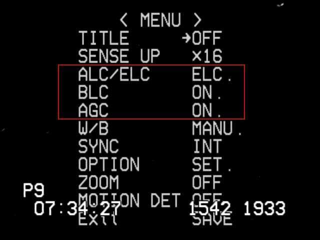
Screen shot of top-level camera settings. The three settings in the red box are NOT set correctly. These settings are particularly bad because they can prevent getting an accurate time for an occultation. The settings should be ALC (SHUTTER OFF, LEVEL to the far right), BLC (OFF), and AGC (MANU, set to the maximum).
First the bad news. There are settings for the camera where the data will look good but you will get very poor timing results. The image to the right shows a mis-configured camera. The incorrect settings in the red box all lead to potentially strange results. What does it do? Well, note the setting here for a sense up of x16. The sense-up setting controls the effective exposure time for the data. In this case each image from the camera is supposed to take 16/59.64 seconds (0.267 seconds). You cannot figure out an accurate disappearance time if you don’t know the exposure time. The automatic modes shown in this bad example have the effect of letting the camera adjust the sense-up setting at any time it likes. The idea here is that with these modes it’s all about getting a pretty picture, not about taking accurate occultation data. This doesn’t always mean the data will be bad. In fact, you can’t really see a problem just visually looking at the screen. It’s only when you extract a lightcurve that you see what’s happening. In principle, if you knew exactly when each exposure happened and what it’s duration is, you can get back to the correct timing. Unfortunately, there is no reliable way to ensure knowing this and the result is that you have to guess in order to analyze the data. I hope I don’t have to spend a lot of time convincing you that guessing is a bad way to do a scientific measurement. The bottom line here is that you must always have these settings set to the recommended standard and fixed values, forcing the camera to operate in the same way throughout the observation.
Now the good news. If you use the suggested settings for the camera, the MallinCAM is capable of taking very good occultation data.
Sensitivity
The second area of concern for the camera is to know how sensitive it is. By this I really mean, what’s the faintest thing that can be seen? Why does this matter? A well-known property of the sky we see is that there are more faint stars than there are bright stars. From star catalogs we know there are 116,000 stars that are 9th magnitude or brighter. Even though that sounds like a lot of stars, there aren’t that many occultations we will see with stars this bright and we’d wait a long time between events if that was as faint as we can see. The situation gets better as you go fainter. For example, there are 6.1 million stars that are 13th magnitude or brighter. By going 4 magnitudes fainter the rate of observable occultations increases by more than a factor of 50. The original baseline plan of RECON was to be able to work on stars this faint. The first order of business was to make sure we can go this faint but it’s also important to know just how faint we can go in case we can go fainter. If we can get to 15th magnitude the number of stars goes up to almost 36 million, or an increase in the rate of occultations by another factor of 6.
The question of sensitivity is much more important than you might think at first glance. In fact, this very question was a central issue in the proposal we submitted to the National Science Foundation in Nov 2013. We had to make a convincing case about just how sensitive our system is and how that translates into how productive our project will be. Obviously, we want to get the maximum amount of return from the invested grant funding.
During all our campaigns in 2013 it became very obvious to me that we could easily work with 13th magnitude stars. That’s really great news but I really did have reason to believe this would be true. The next question to answer is to know how much fainter we can go. This is a harder question to answer from our occultation attempts since we did not try for any really faint stars. In fact, working with faint stars with main-belt asteroid occultations has its own challenges since the asteroids are easily seen by our equipment (as you have seen yourself). With our TNO events, you will never see the TNO itself since it is typically a 23-24th magnitude object. This means we can more easily work with much fainter stars.

Video image of a star field taken by Jerry Bardecker. This image was taken with SENSE-up x128 and a computer-based frame grabber. The red circle is around a 15th magnitude star. The yellow circles are around 13th magnitude stars. The green circle is around an 11th magnitude star. The faintest stars that can be seen here are about 16th magnitude. This field is at J2000 01:00:34.2 +49:44:09.
In November, I sent a request to Jerry to have him take a picture of a patch of sky where there were a lot of stars of varying brightness. By taking a short video of this area in a few different sense-up settings I could then simulate our system performance on occultations of fainter stars. Based on this image we can easily go as faint as magnitude 15. In fact, the true limit is somewhat closer to 16. This is very exciting for the RECON project as it means we will have many more opportunities to work with than I originally estimated. There is, however, one subtle lesson buried here in these test data. That lesson is the subject of the next section. For now, we know that we have a very sensitive camera that can do a really great job on observing occultations.
Data system
The system we’ve been using up to now employs a mini-DVR to record the video data. This unit is pretty convenient and (mostly) easy to use. It was also really, really cheap and as far as I know, 100% of our units are still functional. Ok, that’s the good news. The bad news is that these systems significantly degrade the data coming out of the MallinCAM.
Back in October, I chased an occultation by Patroclus, using the standard RECON system. A few days earlier, Jerry observed an occultation by Dorothea. Jerry’s system is slightly different from the standard RECON system. The most important difference is that he uses a computer with a frame grabber to record the video. This is also used by a few other RECON teams that have computers readily available near their telescopes. I’ve know about frame grabbers and I always knew they were better but the cost and complexity of this setup is somewhat higher and I wanted to stay as simple and cheap as possible.
About this same time, I sent the Susanville camera and data system to an avid IOTA member and occultation chaser, Tony George. Tony volunteered to test out our system to see what he could learn. He did this and distributed a document entitled: Comparison of Canon Elura 80 camcorder to mdvr. The most important thing he did here was to compare a system he understood really well (and works well) against our mini-DVR. He set up a test where he sent the same signal to his recorder and our mini-DVR so the exact same data were record on both. This test eliminates any differences in atmospheric conditions or telescope focus variations. Ideally, one would see the same data in the saved files. Tony has been trying to get me to use the Canon video recorder for quite some time but I don’t like this path because the recorders are no longer manufactured and it requires a second step of playing back the recorder into a computer before the data can be analyzed. I’ve never worried about the data quality since Tony has shown time and time again that his setup is extremely good.
Anyway, the combination of Tony’s report plus the two occultations from October finally made it clear what’s going on. There are two key things at work, both having to do with aspects of the mini-DVR.
Timing
The first issue has to do with the task of converting the video signal to digital images. There’s actually an important clue buried in the two images shown earlier in this post. Video images are a bit more complicated than they appear. The type of video we are working with is called interlaced video, now sometimes called 480i. Video images we get are 640×480 pixels and we get 29.97 such images per second. The normal term is actually frame and I’ll use that here from now on. Each frame is made up of 640 columns of pixels and 480 rows, more commonly called lines but these frames are actually made up of two fields that have 640 columns and 240 lines. These fields alternate between encoding the even rows and the odd rows. Thus, a frame is made up of two adjacent fields where they are interlaced by lines together into a single frame. The field rate is twice as fast as the frame rate with 59.94 fields per second.
Our IOTA-VTI box actually keeps track of all this and will superimpose information on each field as it passes through the box. Look closely at the overlay on the first image above. P9 tells us that 9 (or more) satellites were seen. The next bit is obviously a time, 07:34:27. The next two numbers have always been a little mysterious (only because I didn’t fully absorb the IOTA_VTI documentation). You see 1542 and 1933 toward the lower right. The right-most number, 1933, is the field counter. It increments by one for every field that the IOTA-VTI sees, counting up from 0 starting with the time it is powered on or last reset. The number to the left, 1542, is the fraction of the second for the time of that field. One strange thing I’ve always noticed but never understood is that the middle number can show up in two different places. Thus, looking at this image we can tell that it was passed through the IOTA-VTI box at precisely 07:34:27.1542 UT. This time at the start of the field. Note that it takes 0.017 seconds to transmit this field down the wire so you have to be careful about where in the transmission the time refers to.
The second image looks a little different. Here we see P8 that shows eight satellites were in view by the IOTA-VTI box. Next on the row there is the time, 06:25:50, followed by three sets of digits. Furthermore, the middle two numbers are gray, not white and the last digit of the last number looks messed up. If you look carefully at the full resolution image you see that one of the two gray numbers is only on even rows (lines) and the other is only on odd rows. The last digit can be properly read if you just look at even or odd lines as well. At this point you can see what the VTI box is doing. It is adding different text to each field, first on the odd lines and then on the even lines. When the two fields are combined into a single frame you get this text superimposed on itself. Where it doesn’t change it looks like a normal character. Where it changes you see something more complicated. Armed with this knowledge we can now decipher the timing. This image (frame) consists of one field that started at 06:25:50.0448 and one field that started at 06:25:50.0615 UT.
The question I started asking myself is this: why does the mini-DVR only show one time and why does the frame grabber show two? Tony’s report showed me the answer. The mini-DVR only records one field per frame. Internally, the mini-DVR only samples one field and it can either be the even or odd field. It then copies the field it got to the other field making a full frame. This saves time for the recorder since it has to take the frame and then process it and write it out to the memory card. I’ll have a lot more to say about the processing it does in the next section. For now, it is sufficient to realize that only half of the image data coming out of the camera actually makes it to the video file. In terms of the occultation lightcurve, this is equivalent to cutting down the size of our telescope to an 7.88-inch aperture, alternatively it means we lose nearly a magnitude in sensitivity. In a frame-grabber system, you get all of the data.
Data quality
Recall that I said the mini-DVR has to process the frames before saving the data to the memory card. The most important thing that happens here is data compression. Even 480i video data generates a lot of data. The camera is generating 307,200 bytes of data for every frame. It’s actually worse at the DVR since it interpret the black and white images as color, making the effective data rate three times higher. This amounts to just over 26 Mbytes of data per second. In only three minutes you generate enough data to fill a DVD (roughly 4Gbytes total capacity). In six minutes you would fill up our 8Gb memory cards. This data rate is a problem for everyone, including movie studios that want to cram a 3 hours movie onto one DVD. The fix is to use data compression. A lot of effort has gone into this and there are some pretty good tools for this. However, the best tools can take a long time to do the compression and in our systems you don’t have much time. Our cheap little mini-DVR has just 0.017 seconds to compress and save each frame and that’s a pretty tall order. In fact, that’s why the DVR throws away every other field. It has to, otherwise there isn’t enough time to process the data. This compression can be sped up a lot but a consequence of the compression method chosen is that it must throw away information (that’s called lossy compression). Once thrown away you can never get it back. Another trick the DVR uses is to darken the image just a bit. In doing so, the sky in the image is set to all black and that makes the compression even more effective. The result of all this is that we get comparatively small files, like 20-30Mb. Those sites using frame grabbers are typically uploading much larger files, like a few Gb.
This compression turns out to cause problems with our data as well. The consequences aren’t as obvious but everything degrades the timing accuracy of our system. In comparison, a frame grabber system will typically get timings better than 0.01 seconds while the mini-DVR could be as bad as one second with no way to know how large the real error is. When you put all of these effects together, it says that the mini-DVR is not a very good choice for our project. It does work, but, we can get more out of our telescope and camera and increase our scientific productivity by doing something better.
The next step
One obvious fix is to find a better mini-DVR. Sadly, getting a better recorder at this price is just not an option. There are digital recorders that can do this but they are way too expensive for this project. An alternative is to switch to using a frame-grabber system. Since learning these lessons I have been testing a computer based data acquisition system. I tried two low-cost netbook computers with an inexpensive USB to video adapter. Both of the netbook options work just fine once you get them configured right. The bottom line is that for about $350 we can move to a computer system for recording the data. That’s about $300 more than the DVR solution but the improvement in the data quality is worth it.
The plan now is to get computers for those sites that aren’t already using them, and move to getting rid of the mini-DVRs. This upgrade has been incorporated into the budget for the new proposal but I am looking at ways to speed up the process for the current RECON sites. It will mean learning some new procedures and it will significantly increase the time it takes to upload the data but the results will be well worth the effort.