Check out the following post about our project. Subscribe to my occsci substack (it’s free) if you want to get more news and information about occultations.

Check out the following post about our project. Subscribe to my occsci substack (it’s free) if you want to get more news and information about occultations.
Congratulations to all of you that have been a part of RECON. It’s been six years since we began the pilot project and four years since the start of the full project. We’ve all learned a lot together and it’s been an amazing project throughout. We are known in the scientific community throughout the world for our work on the Kuiper Belt.
While we’ve been hard at work, the rest of our colleagues have also been probing the boundaries of knowledge of the outer solar system. Rings around tiny Centaur objects! Maybe a Planet X out there (or maybe not). Binary objects remain an important component of these objects and it’s widely recognized that RECON is the perfect tool to expand that study.
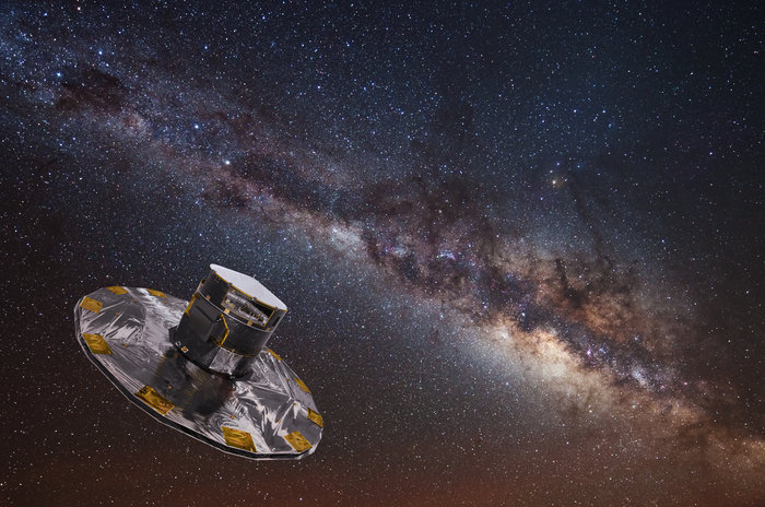
Artist representation of Gaia spacecraft. Credit: ESA.
The Gaia mission from the European Space Agency has delivered on its promise to pin down where a huge number of stars are. As I’ve talked about many times, this is essential to the long-term success and productivity of RECON and any other occultation-based study of objects in our solar system. It took a couple of extra years to get to this point but we are now starting to see the benefits enabled by Gaia. In the early days of the project we were limited a bit by having to work with a much less accurate star catalog and also much poorer knowledge of the positions of the TNOs. The explosion of occultation opportunities is now upon us.
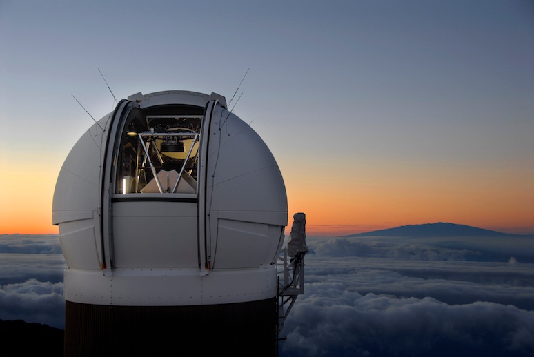
PanSTARRS – Panoramic Survey Telescope And Rapid Response System. Credit: IFA
Within the project we have continued to work on measuring where candidate TNOs are to help increase the number of good events to observe. That work continues but we are now working closely with the PanStarrs survey in Hawaii. Their dataset is an amazing resource that has, in the past few months, provided thousands of observations of more than a hundred objects. With the telescopes we have available ourselves, this contribution would take us 300 nights of observing on giant telescopes to equal.
A good example of this is our campaign observation for RECON of the TNO 2014TA86. This object was discovered in 2014 by PanStarrs and the recent effort located nearly 10 years of data that had already been collected on this object by PanStarrs but not yet processed. As a result we know where this object is with much more precision that is usual for something discovered in 2014. Without the support from PanStarrs, we wouldn’t even know this object existed and now we are poised to make critical measurements of its size and position. If it turns out to be binary (which is quite likely), we’ll be adding more to our understanding of these distant worlds. Note that the shorter than usual notification of the impending campaign was a result of this recent data dump from PanStarrs coming in. This event popped up in our scans, and it was just too good to pass up, so we made an exception to our normal procedure of providing a month’s notice.
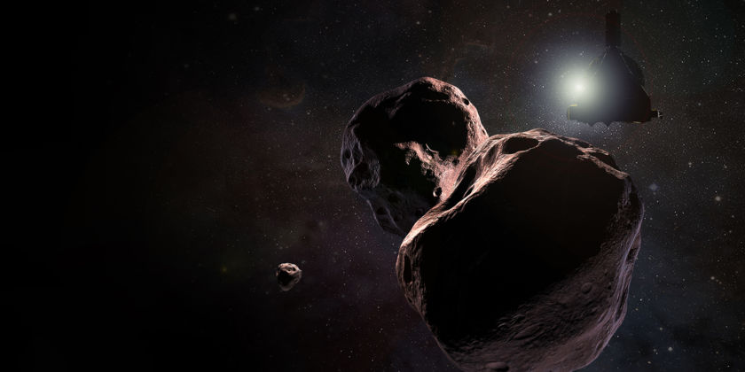
Artists depiction of MU69. Credit: NASA
The context of our efforts is greatly expanded with the historic event to come on Jan 1, 2019. New Horizons will have a close flyby of (486958) 2014MU69, a TNO that I discovered by in 2014. It’s a neighbor of this month’s campaign target and whatever we learn from New Horizons will provide a broader understanding of our RECON target. What’s even more exciting is that our observations will provide a broader understanding of the New Horizons data as well.
I’m very excited to see what we will learn from New Horizons. I’ve been unbelievably busy this year and last organizing and chasing occultations by MU69. Many of the lessons learned with RECON were a key to the success of those occultation expeditions. I sent 25 teams of astronomers out on three separate occasions. South Africa, Argentina, Senegal, and Colombia were all visited by these dedicated teams of astronomers, braving clouds, storms, high winds, mosquitoes, insane urban traffic, and more. It was an exhausting, yet fulfilling effort, and the team work was truly amazing. All of you that have been a part of RECON can take pride in knowing that you helped make these other efforts a success.
Now it’s our turn. Early in the morning, on Friday, October 12, we will have a shot at our own historic observation of this distant TNO. What will we find? Should we let a minor inconvenience like having to get up in the middle of the night, during the week, to get in our way of learning more about our solar system? I’ve said all along in this project that astronomy isn’t always at a convenient time. We’ll continue the fine tradition of making a special effort to learn more about the universe around us. I’ll be observing from home along with all of you to add my own efforts but you are all truly the stars of the project. I should also warn you that we’re looking at a lot of very nice opportunities in the coming six months during our peak season. It will be RECON like never before. How exciting!
I was practicing for a RECON campaign the other evening. Everything was up and running and my first alignment of the night was a quick success. At that point I sent the telescope off to the first RECON field of the night. After getting there I needed to change the camera setting to a senseup of x128. When I touched the camera housing I felt the tiniest of a static electricity spark leap from my finger to the camera. That’s very unusual but it was a really dry day.
Here’s the thing: at the instant I felt the spark the sound of the telescope drive motors changed pitch and volume by a little bit. Of course, the telescope is tracking and it makes its quiet humming sound as it works. An abrupt change like that got my spidey-senses tingling but there didn’t seem to be any major problems except I saw the telescope was no longer tracking perfectly. I was seeing a very slow but inexorable drift of the field on the camera image. Not good, but I still wasn’t sure there was much of a problem. But, better safe than sorry. I decided to redo the pointing.
Well, redoing the pointing wasn’t helping at all. I tried three times in a row, changing stars each time and by the end I knew that something was very wrong. I’m at least one of those attempts should have worked. Rather than try, try again without changing anything, I decided I would start all over again. That means turning off the power to the telescope and letting it sit a minute. After I turned it back on I was quickly able to get a good alignment and quickly found the RECON campaign field. So what happened?
I think the static spark caused the GPS information (time or position) to be corrupted. My theory is that this information is loaded at the very start and isn’t updated again. After the spark, either a bad position or time meant the computer was doomed to failure since the stars would never appear to be in the right place. That would also make tracking and pointing all wrong. The odd thing is that the telescope, camera, and computer all thought everything was fine.
This experience is worth sharing as an example of one way things can go wrong and how to recover. The key, as always, is to 1) know your equipment and that means practice, and 2) pay attention to your equipment and what it’s telling you when in use. I never would have thought a static spark could do this but that myth has now been dispelled. I wonder how many of you have been inadvertently bitten by this failure mode. I suspect this will only happen when it is very, very dry out and even then will still be rare. In my case, the relative humidity was below 10% and I only got that one little spark the entire night. I sure am glad it wasn’t just before an actual campaign event!
A couple of teams have had problem with their laptops that were very puzzling. In this case, a working computer became non-functional and unresponsive. The initial guess was a dead battery but the machines were reported to have been “plugged in all day”. It turns out that the problem is a bit of confusion over the proper power supply for the laptop. The power connector for the laptop happens to be essentially the same as the rest of the barrel connectors for the other equipment. The correct power supply for the laptop provides 19V power. Everything else provides 12V.
The confusion centers on the extra power supply provided with your MallinCAMs. In normal circumstances we don’t use this. A picture of one of these power supplies is shown below:

MallinCAM power supply. This unit provides 12V power. It is not normally used but can be useful for indoor testing.
There are two versions of the CORRECT power supply shown below. Which charger you have depends upon which batch of laptops you received, but both versions have a transformer that is labeled with an output value of 19V. The first version has a removable plug at the transformer end that can be rotated if your wall plug or power strip doesn’t like the orientation you are using The second version has a removable cord at one end of the transformer that goes to 110V power.
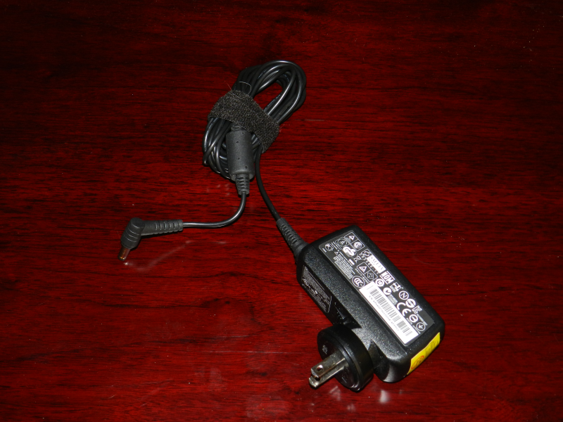
One correct version of the Laptop power supply. This unit provides 19V power, as labeled on the transformer.
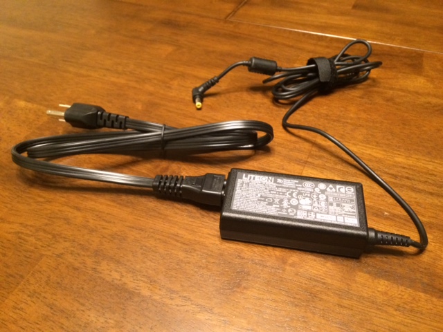
A second correct version of the Laptop power supply. This unit provides 19V power, as labeled on the transformer.
As always, the computer will actually tell you if it is charging properly. There is a little red light on the front of the machine that you can see even with the lid closed. Red means it is charging. While running, there is a tool on the task bar that will tell you if you are on battery or wall power.
To date in the project we have been using a mini-DVR for recording video for our occultation events. In my last posting, I talked about the problems discovered with this approach. Since then I have been working on setting up a new data recording system. This week marks the completion of that work and new data collection tools will be shipped out to all the teams. This document discusses the changes and the reasoning. New training documents will also be made available shortly to help with the transition.
We are going to now use netbook computers in the field for data collection. I tried a couple of different systems and settled on an Acer Aspire V5 running Windows 7. These systems will come pre-configured with VirtualDub, OccultWatcher, LiMovie, Chrome, LibreOffice, Skype, Occult, and a few other useful utilities. These computers should not be used for general tasks, instead they are project machines for things like collecting data, transmitting data to SwRI, and signing up for events. A small amount of customization of each system will be required, such as putting in your OW credentials.
Each computer comes with a video frame grabber interface (StarTech SVID2USB2) and a video cable that will connect to the output of the IOTA-VTI box. Inside the box are also a couple of spare fuses as well as some of our cool new RECON stickers. I recommend using at least a few of these stickers on the equipment (telescope, telescope crate, and so on). If you need more, let me know.
I think you will all like the new system. It’s not so great for dark adaption, the screen seems really bright at night even turned all the way down. But, you’ll be able to get a bigger image on the screen than what’s been possible with the mini-DVR and you’ll find that focusing and finding the field will be easier since you can see it from a distance while operating the telescope. The program, VirtualDub, is what you run to see the video signal coming in. Once you turn on the capture mode the video is live. Stay tuned for a more detailed document on how best to setup and use this program.
The data quality from this setup is exceptionally good. There is a price, however. The files you have been collecting with the mini-DVR up to now are really quite small. The new system makes much bigger files. The data rate is about 200Mb/minute and your upload times will be significantly longer. Unfortunately, this can’t be helped but the extra time will pay off in the increased scientific value of the data. Note that the data are compressed pretty well already. You won’t get much more out of using zip other than to pack a bunch of files into one clump for a single upload.
Everyone should see their systems arriving late this week or early next week. I’m trying to get this equipment in your hands in advance of the 2001XR254 event in early March. I’m confident you’ll be able to make the switch in time but in an emergency the mini-DVR will be able to handle this upcoming event.
2013 has been an amazing year for the RECON project. We’ve progressed from an idea to a community in this short period of time. One element of this effort is to better understand our observing system. Central to that need is our camera and the data system (miniDVR). This posting is a summary of lessons learned with plans about where we’re headed in the future.
As you know, we have been using the MallinCAM B&W Special. My earlier testing indicated this would be a good camera for us but it remained to collect actual data and understand this device in gory detail. Thanks to all team members I have enough information in hand to answer most of my burning questions. I would like to specially thank Jerry Bardecker (RECON-Gardnerville) for his help in taking test data on short notice and two students from Berthod High School, Jo and Melody, who helped with laboratory-based timing tests.
One of the most important measurement goals of our project is to accurately time the disappearance and reappearance of the stars as they are occulted by an asteroid. There have been numerous rumors floating around the occultation community that the MallinCAMs had some strange timing issues. The answer, as with all real research projects, turns out to be complicated. There’s good news and there’s bad news.
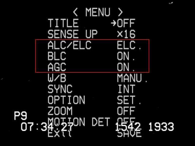
Screen shot of top-level camera settings. The three settings in the red box are NOT set correctly. These settings are particularly bad because they can prevent getting an accurate time for an occultation. The settings should be ALC (SHUTTER OFF, LEVEL to the far right), BLC (OFF), and AGC (MANU, set to the maximum).
First the bad news. There are settings for the camera where the data will look good but you will get very poor timing results. The image to the right shows a mis-configured camera. The incorrect settings in the red box all lead to potentially strange results. What does it do? Well, note the setting here for a sense up of x16. The sense-up setting controls the effective exposure time for the data. In this case each image from the camera is supposed to take 16/59.64 seconds (0.267 seconds). You cannot figure out an accurate disappearance time if you don’t know the exposure time. The automatic modes shown in this bad example have the effect of letting the camera adjust the sense-up setting at any time it likes. The idea here is that with these modes it’s all about getting a pretty picture, not about taking accurate occultation data. This doesn’t always mean the data will be bad. In fact, you can’t really see a problem just visually looking at the screen. It’s only when you extract a lightcurve that you see what’s happening. In principle, if you knew exactly when each exposure happened and what it’s duration is, you can get back to the correct timing. Unfortunately, there is no reliable way to ensure knowing this and the result is that you have to guess in order to analyze the data. I hope I don’t have to spend a lot of time convincing you that guessing is a bad way to do a scientific measurement. The bottom line here is that you must always have these settings set to the recommended standard and fixed values, forcing the camera to operate in the same way throughout the observation.
Now the good news. If you use the suggested settings for the camera, the MallinCAM is capable of taking very good occultation data.
The second area of concern for the camera is to know how sensitive it is. By this I really mean, what’s the faintest thing that can be seen? Why does this matter? A well-known property of the sky we see is that there are more faint stars than there are bright stars. From star catalogs we know there are 116,000 stars that are 9th magnitude or brighter. Even though that sounds like a lot of stars, there aren’t that many occultations we will see with stars this bright and we’d wait a long time between events if that was as faint as we can see. The situation gets better as you go fainter. For example, there are 6.1 million stars that are 13th magnitude or brighter. By going 4 magnitudes fainter the rate of observable occultations increases by more than a factor of 50. The original baseline plan of RECON was to be able to work on stars this faint. The first order of business was to make sure we can go this faint but it’s also important to know just how faint we can go in case we can go fainter. If we can get to 15th magnitude the number of stars goes up to almost 36 million, or an increase in the rate of occultations by another factor of 6.
The question of sensitivity is much more important than you might think at first glance. In fact, this very question was a central issue in the proposal we submitted to the National Science Foundation in Nov 2013. We had to make a convincing case about just how sensitive our system is and how that translates into how productive our project will be. Obviously, we want to get the maximum amount of return from the invested grant funding.
During all our campaigns in 2013 it became very obvious to me that we could easily work with 13th magnitude stars. That’s really great news but I really did have reason to believe this would be true. The next question to answer is to know how much fainter we can go. This is a harder question to answer from our occultation attempts since we did not try for any really faint stars. In fact, working with faint stars with main-belt asteroid occultations has its own challenges since the asteroids are easily seen by our equipment (as you have seen yourself). With our TNO events, you will never see the TNO itself since it is typically a 23-24th magnitude object. This means we can more easily work with much fainter stars.

Video image of a star field taken by Jerry Bardecker. This image was taken with SENSE-up x128 and a computer-based frame grabber. The red circle is around a 15th magnitude star. The yellow circles are around 13th magnitude stars. The green circle is around an 11th magnitude star. The faintest stars that can be seen here are about 16th magnitude. This field is at J2000 01:00:34.2 +49:44:09.
In November, I sent a request to Jerry to have him take a picture of a patch of sky where there were a lot of stars of varying brightness. By taking a short video of this area in a few different sense-up settings I could then simulate our system performance on occultations of fainter stars. Based on this image we can easily go as faint as magnitude 15. In fact, the true limit is somewhat closer to 16. This is very exciting for the RECON project as it means we will have many more opportunities to work with than I originally estimated. There is, however, one subtle lesson buried here in these test data. That lesson is the subject of the next section. For now, we know that we have a very sensitive camera that can do a really great job on observing occultations.
The system we’ve been using up to now employs a mini-DVR to record the video data. This unit is pretty convenient and (mostly) easy to use. It was also really, really cheap and as far as I know, 100% of our units are still functional. Ok, that’s the good news. The bad news is that these systems significantly degrade the data coming out of the MallinCAM.
Back in October, I chased an occultation by Patroclus, using the standard RECON system. A few days earlier, Jerry observed an occultation by Dorothea. Jerry’s system is slightly different from the standard RECON system. The most important difference is that he uses a computer with a frame grabber to record the video. This is also used by a few other RECON teams that have computers readily available near their telescopes. I’ve know about frame grabbers and I always knew they were better but the cost and complexity of this setup is somewhat higher and I wanted to stay as simple and cheap as possible.
About this same time, I sent the Susanville camera and data system to an avid IOTA member and occultation chaser, Tony George. Tony volunteered to test out our system to see what he could learn. He did this and distributed a document entitled: Comparison of Canon Elura 80 camcorder to mdvr. The most important thing he did here was to compare a system he understood really well (and works well) against our mini-DVR. He set up a test where he sent the same signal to his recorder and our mini-DVR so the exact same data were record on both. This test eliminates any differences in atmospheric conditions or telescope focus variations. Ideally, one would see the same data in the saved files. Tony has been trying to get me to use the Canon video recorder for quite some time but I don’t like this path because the recorders are no longer manufactured and it requires a second step of playing back the recorder into a computer before the data can be analyzed. I’ve never worried about the data quality since Tony has shown time and time again that his setup is extremely good.
Anyway, the combination of Tony’s report plus the two occultations from October finally made it clear what’s going on. There are two key things at work, both having to do with aspects of the mini-DVR.
The first issue has to do with the task of converting the video signal to digital images. There’s actually an important clue buried in the two images shown earlier in this post. Video images are a bit more complicated than they appear. The type of video we are working with is called interlaced video, now sometimes called 480i. Video images we get are 640×480 pixels and we get 29.97 such images per second. The normal term is actually frame and I’ll use that here from now on. Each frame is made up of 640 columns of pixels and 480 rows, more commonly called lines but these frames are actually made up of two fields that have 640 columns and 240 lines. These fields alternate between encoding the even rows and the odd rows. Thus, a frame is made up of two adjacent fields where they are interlaced by lines together into a single frame. The field rate is twice as fast as the frame rate with 59.94 fields per second.
Our IOTA-VTI box actually keeps track of all this and will superimpose information on each field as it passes through the box. Look closely at the overlay on the first image above. P9 tells us that 9 (or more) satellites were seen. The next bit is obviously a time, 07:34:27. The next two numbers have always been a little mysterious (only because I didn’t fully absorb the IOTA_VTI documentation). You see 1542 and 1933 toward the lower right. The right-most number, 1933, is the field counter. It increments by one for every field that the IOTA-VTI sees, counting up from 0 starting with the time it is powered on or last reset. The number to the left, 1542, is the fraction of the second for the time of that field. One strange thing I’ve always noticed but never understood is that the middle number can show up in two different places. Thus, looking at this image we can tell that it was passed through the IOTA-VTI box at precisely 07:34:27.1542 UT. This time at the start of the field. Note that it takes 0.017 seconds to transmit this field down the wire so you have to be careful about where in the transmission the time refers to.
The second image looks a little different. Here we see P8 that shows eight satellites were in view by the IOTA-VTI box. Next on the row there is the time, 06:25:50, followed by three sets of digits. Furthermore, the middle two numbers are gray, not white and the last digit of the last number looks messed up. If you look carefully at the full resolution image you see that one of the two gray numbers is only on even rows (lines) and the other is only on odd rows. The last digit can be properly read if you just look at even or odd lines as well. At this point you can see what the VTI box is doing. It is adding different text to each field, first on the odd lines and then on the even lines. When the two fields are combined into a single frame you get this text superimposed on itself. Where it doesn’t change it looks like a normal character. Where it changes you see something more complicated. Armed with this knowledge we can now decipher the timing. This image (frame) consists of one field that started at 06:25:50.0448 and one field that started at 06:25:50.0615 UT.
The question I started asking myself is this: why does the mini-DVR only show one time and why does the frame grabber show two? Tony’s report showed me the answer. The mini-DVR only records one field per frame. Internally, the mini-DVR only samples one field and it can either be the even or odd field. It then copies the field it got to the other field making a full frame. This saves time for the recorder since it has to take the frame and then process it and write it out to the memory card. I’ll have a lot more to say about the processing it does in the next section. For now, it is sufficient to realize that only half of the image data coming out of the camera actually makes it to the video file. In terms of the occultation lightcurve, this is equivalent to cutting down the size of our telescope to an 7.88-inch aperture, alternatively it means we lose nearly a magnitude in sensitivity. In a frame-grabber system, you get all of the data.
Recall that I said the mini-DVR has to process the frames before saving the data to the memory card. The most important thing that happens here is data compression. Even 480i video data generates a lot of data. The camera is generating 307,200 bytes of data for every frame. It’s actually worse at the DVR since it interpret the black and white images as color, making the effective data rate three times higher. This amounts to just over 26 Mbytes of data per second. In only three minutes you generate enough data to fill a DVD (roughly 4Gbytes total capacity). In six minutes you would fill up our 8Gb memory cards. This data rate is a problem for everyone, including movie studios that want to cram a 3 hours movie onto one DVD. The fix is to use data compression. A lot of effort has gone into this and there are some pretty good tools for this. However, the best tools can take a long time to do the compression and in our systems you don’t have much time. Our cheap little mini-DVR has just 0.017 seconds to compress and save each frame and that’s a pretty tall order. In fact, that’s why the DVR throws away every other field. It has to, otherwise there isn’t enough time to process the data. This compression can be sped up a lot but a consequence of the compression method chosen is that it must throw away information (that’s called lossy compression). Once thrown away you can never get it back. Another trick the DVR uses is to darken the image just a bit. In doing so, the sky in the image is set to all black and that makes the compression even more effective. The result of all this is that we get comparatively small files, like 20-30Mb. Those sites using frame grabbers are typically uploading much larger files, like a few Gb.
This compression turns out to cause problems with our data as well. The consequences aren’t as obvious but everything degrades the timing accuracy of our system. In comparison, a frame grabber system will typically get timings better than 0.01 seconds while the mini-DVR could be as bad as one second with no way to know how large the real error is. When you put all of these effects together, it says that the mini-DVR is not a very good choice for our project. It does work, but, we can get more out of our telescope and camera and increase our scientific productivity by doing something better.
One obvious fix is to find a better mini-DVR. Sadly, getting a better recorder at this price is just not an option. There are digital recorders that can do this but they are way too expensive for this project. An alternative is to switch to using a frame-grabber system. Since learning these lessons I have been testing a computer based data acquisition system. I tried two low-cost netbook computers with an inexpensive USB to video adapter. Both of the netbook options work just fine once you get them configured right. The bottom line is that for about $350 we can move to a computer system for recording the data. That’s about $300 more than the DVR solution but the improvement in the data quality is worth it.
The plan now is to get computers for those sites that aren’t already using them, and move to getting rid of the mini-DVRs. This upgrade has been incorporated into the budget for the new proposal but I am looking at ways to speed up the process for the current RECON sites. It will mean learning some new procedures and it will significantly increase the time it takes to upload the data but the results will be well worth the effort.
For those of you that tried Isolda, thank you. Seems like most of us had one difficulty or another but it’s good to get that our of our collective systems early. I haven’t had a chance yet to review all of the files uploaded. I really have to get this automated more. Being on the road non-stop isn’t helping either. Last week I was in Flagstaff for a Planetary Defense Conference. Saturday I was at the bottom of Meteor Crater. Today I’m in Baltimore serving on an advisory committee for the Hubble Space Telescope.
I wanted to share some reflections on last week’s Isolda occultation event. First, I have to apologize for one of my mistakes here. I didn’t check on the Moon for this event. It was really close and pretty bright on event night. It gave me a lot of trouble with getting setup and finding the field. I was not really able to use anything on the star hop list fainter than Alhena. If it wasn’t for PreciseGoTo I would not have found the field at all. In the end, the moonlight caused me to take longer than anticipated to get on the field and I was very rushed for time to get the data recorder started.
Aside from the obvious reminder lessons floating around that night, I learned something really important about our cameras. The concept is a little tricky to explain but the bottom line is that if you use an exposure time (senseup) that is too short, you can fail to detect your object at all. That meant x12 was a really bad idea. Kudos to the Carson City folks in figuring this out and running with x48 instead.
Here’s the details in case you are wondering. I took a lot of data a couple of weeks ago getting ready for the Pluto event. Normally you can take an image with one set of camera parameters and then scale to what you’d expect to see at other settings. I do this all the time, even for working with the Hubble Space Telescope. In our case, this calculation doesn’t quite work right, as I found out. You see, today’s digital detectors are a lot more capable than cameras were at the time the video signal standard (NTSC in the US) was developed. Video is designed for a fairly limited range in brightness, far less than what a good camera can deliver. That means you have to do something in the electronics to match the camera signal to the video output. This is normally labeled “brightness” and “contrast”, same as you’d see on an old TV.
If you were designing the perfect system, there would be a control that would let you set the signal level for the background of your image. There’s always some background, either it’s from the sky brightness directly or it’s from the noise floor of your detector. Now, you can think of a video signal as having 256 levels of brightness — 0 would be black, 128 would be grey, 255 would be white and you have shades in between. I always prefer to see my background. That means I’d set the background to be a signal of 5 to 10, depending on how noisy it is. That means any source in the sky you can detect will be seen as a brighter bump on the background.
Our MallinCAMs have other ideas about how to set the background, unfortunately. Now, I have to say that there’s a chance I just haven’t figured out how to configure them to do what I want but with my current recommended settings this is a problem to watch out for. As I was saying, the MallinCAM doesn’t have a problem with black sky (signal=0). That’s what I had for the Isolda event. The problem with this is that you can’t tell the difference between a signal level of -100 and -1. It all comes out as 0. So, not only could I not see the sky but the star to be occulted was at a signal level below 0 and I only got a few of the brightest stars in my field.
How do we deal with this issue? I’m not entirely sure yet. I can say that x64 for the upcoming Pluto event is safe. I really need to characterize the camera better so I know how to better predict its output. This will be an ongoing effort in the coming months. All of you could help if you like and I’ve also got a couple of bright high school students that are going to work on tasks like this as soon as school lets out.
Oh yes, there’s one other thing that I’ve noted. The DVR screen makes your images look darker and less useful than they really are. I put an example of this on the Pluto event page. This makes it a little tricky to ensure that you are really seeing the sky level when you are in the field.
Portola RECON member Warren asked for more details about how I go from images to orbits for the TNOs we’re interested in. Let me explain.
Most people know that planets, asteroids, and TNOs all orbit the Sun. The force of gravity keeps everything bound together into what we know as the solar system Remember about Kepler and Newton? From their work we have a mathematical theory that describes motion under the force of gravity. If you have just two objects, like the Sun and a single TNO, this simple theory can perfectly describe the motion of these two, forever. The path the TNO takes through space is called its orbit. Now, in our case, we really care more about the mathematical description of its motion. Kepler’s mathematical formalism requires the determination of six parameters at some specific time. Those parameters collectively are known as orbital elements and consist of the semi-major axis, eccentricity, inclination, longitude of the ascending node, longitude of perihelion, and the mean anomaly. From these values it is possible to calculate where an object is at any time.
Ok, so that’s the perfect setup. What’s it like in real life? First of all, you can’t just divine or even directly measure any of the orbital elements. Second, there are far more than two objects in our solar system. Here’s where it starts to get tricky (and sometimes interesting, but that’s a story for another day). Let’s just worry about the first part for now. What can we measure? Well, our most useful instrument is a camera. With this we get an image of the sky that contains stars, galaxies, and perhaps our TNO at some known time and from some known location. Most, if not all, of the stars and galaxies will be objects whose positions are already known. These are known as catalog objects and are used as positional references. Using the catalog objects we can calibrate the correspondence between a position in the image to the coordinates on the sky (known as the celestial sphere). Most of the time this is rather simple. You work out the angular scale of the
image (arc-seconds per pixel) and the sky coordinate of the center of the image. From that you can then calculate the sky coordinate of any pixel. When you work with wide-field cameras there are often distortions in the image that need to be mapped out. Ok, so you see you TNO on the image and then compute its position. This position, known as right ascension and declination, is a pair of angles measured from a single reference point on the sky.
Having a single position is not good enough yet to compute an orbit. Not only do you need to know where it is but you also need to know its velocity (speed and direction). With perfect data, you could simply wait some time from your first picture and then take another. These two positions now give you a measure of the velocity. There’s a
catch, though. First, you never have perfect data. That means your limited in what you can learn in just two measurements. There’s something you cannot easily measure from just two positions. On the sky you get a good measurement of the sky position and the velocity as seen in the sky. You do not have good information on how far away it is or how fast it
is moving toward or away from you. A clever guy named Vaisala figured out a trick for working with limited data like this. His trick was to guess what distance the object is at and you guess that it’s currently at perihelion. Perihelion is when the object is at its closest distance from the sun during its orbit. Unfortunately, with just two points there are lots of guesses that will give you a reasonable orbit but you don’t yet know which is right. Still, it can help you to pick something reasonable that can be used to predict where it will be the next few nights.
As you continue to make measurements (more images at later times), you build up what is called the “observational arc”. Formally, this is the time between your first measurement and your last measurement. As this time gets longer, you can get better and better quality orbits. By that I mean the orbit you think you have gets closer and closer to the true orbit. Now, what about that second thing I mentioned before? Right, there are other things around than just the sun and the one TNO. That means the position and velocity of everything in the solar system depends slightly on the position of all the other objects in the solar system. To get a perfect description you really need to have a catalog that is 100% accurate and complete. This isn’t very likely so we’re resigned to always having orbits that are really just approximations. Are these good enough? In most cases, all you want to do is to find a TNO in your telescope again. That’s the easiest condition to meet. If you want to see an occultation of a star by a TNO we need a very precise orbit. Finally, if you want to send a spacecraft to a TNO we need something extremely good.
You can make your orbits better in different ways. The easiest is to simply wait and then take another picture. Bit by bit as time marches on you will get a better and better orbit. How long you have to wait for a good orbit depends on where the object is in the solar system. Objects closer to the Sun move faster and in so doing let you get a good orbit more quickly than a slow moving object. For a main-belt asteroid orbiting between Mars and Jupiter you generally get an excellent orbit (good for occultations) in just 4-5 years. Note that the one thing that does you no real good is to just take lots and lots of pictures. Time is a lot more valuable than the number of measurements. In fact, on a single night you get the same information from 2-4 observations as you would from a thousand in one night. In the early days after discovery you need to observe more often but then things spread out considerably. One rule of thumb I use is the “rule of doubling”. This rule says that you want to wait twice as long as your current observational arc before you both to measure it again. Here’s an example: you find a new TNO on some night with two images that are one hour apart. The third image should be three hours after the first image. The fourth should be at 6 hours, the fifth at 12, then at 1 day, 2 day, 4 day, 8 day, 16 day, 32 day, and so on. After a while you are waiting years or even decades for that factor of two. Now, this really isn’t a rigorous rule, after all, the Sun keeps coming up making it hard to see your object. Still, if you followed this rule you would never lose a newly discovered object.
Another way to get better orbits if you are impatient is to use a more accurate catalog. The quality of your positions for your TNO is only as good as your catalog. If you use a better catalog you get better positions. The problem is that this is really hard to do. We’ve got really good catalogs now but they could be a lot better. In fact, there is a European mission, named Gaia and planned for launch later this year, that will measure all the star positions to an unprecedented accuracy. I can’t say enough about this mission. It will completely revolutionize occultation observations by making it very easy to predict where the asteroid shadows will fall. Alas, it’s going to be quite a few years before these results are available and work their way into better TNO positions.
A third way that works really well is to use radar. The Arecibo and Goldstone radio telescopes are used for this with near-Earth asteroids where they bounce a signal off the asteroid and analyze the return signal. Radar is especially valuable because it can directly measure distance to the target and how fast it is moving toward or away from us. The problem is that the objects have be close. It’s just not practical to use this method on a TNO.
Now, think about sitting at the telescope and trying to get better orbits. That’s what I was doing in March, 2013. I have information on every measurement ever made of a TNO (asteroids too, for that matter) and I know something about how good the orbit is. I’m looking for objects whose positions are poorly predicted that have not been seen in a while. This is a very complicated thing to do at the telescope and I have some very powerful software that helps me keep track of what I’ve done and what I might be able to do as the night goes on. I can say that 3 clear nights on a big telescope can be a very exhausting experience but well worth the effort. Then, once the night is over there is the task of getting the positional measurements off the images. I’ll leave that discussion for another time.
The Isolda event is tomorrow night for those of you interested. I note that we’ve got one RECON site signed up for this. I’m currently in Flagstaff and I will attempt the event as well, weather permitting. The forecast here is for clearing conditions. I’m waiting until closer to event time before signing up for a location to see who else will give it a try (IOTA or RECON). If you do intend to observe this you really need to sign up on OW. As more show up, the IOTA folks will hopefully treat it more seriously. I posted a message to the IOTAoccultations group to try and drum up interest.
This event will be very interesting even if we only have a few of us doing it provided we also get some IOTA members to participate. We will get our first chance to compared timing results from our cameras to the more well-tested systems that IOTA uses.
On the event page I have recommended a senseup setting of x12. I have not actually used this on the field but instead have estimated the setting from other test data I’ve taken. If I did this right the star will be there but not terribly bright in the image you’ll see. If you just can’t see it, go slower to make sure but this is a good starting point. I would like to ask those of you trying this with larger telescopes (12″ or 14″) to use a slightly faster senseup setting. On a 12″ x10 would be the same as x12 on an 11″. I don’t remember if there is an x10 setting or not, though. If not, use x12. For a 14″, x8 would be equivalent. I think that’s a valid setting. I’m interested in getting chords with different senseup settings to see if there is a change in the timing we extract that depends on the sense up setting.
These have been busy days since the Kitt Peak observing run. Those observations are critical for us to help find interesting occultation events to try but they are of no use in the form of images. But that comment I mean that the easy part is over once the pictures are taken. There’s a lot of image processing and analysis that is required. I have to calibrate the images as well as map the sky coordinates. After that I have to scan the images looking for all the moving things. Most of the moving objects are main-belt asteroids but a few of them are the slow-moving Kuiper Belt objects that are our targets. Once all these objects are found I then extract their positions and use that information to improve the orbits. Good orbits are the key to letting me predict where these things will be at some future time.
This work, while difficult and time consuming, is made easier by the software that I’ve developed over the past 15 years. One of the nasty realities in professional astronomy is that there is very little standardization in the data I get. Usually, I can count on data from the same camera having the same data format. But, this observing run was with a camera that I’ve never used before. Even though this camera is on a telescope I’ve used, the data are just different enough that I had to rework a lot of my software. In the process, I discovered that there was a serious problem in the supporting data. One of the key bits of information I need to know is exactly when each picture was taken. Without a good time, the observations are useless for our project. Well, it turns out the times recorded by the camera was incorrect and off by as much as 12 minutes. That may not sound like a lot to you but to me it’s huge. Want to know how I figured this out?
Well, it’s like this. Time on telescopes like this is very precious and I work very hard during my nights to make sure that I’m getting as much data as possible. The ideal thing would be to be collecting light 100% of the time. Unfortunately, there are unavoidable times when you can’t collect light. After each picture we have to stop and read out the image and save it to the computer disk. This camera is quite fast and can store the 16 mega-pixel image in about 25 seconds. Not as fast as a commercial digital camera but then it’s much more precise and getting that precision requires a little extra time. Now, each picture takes about 4 minutes to collect (that’s when the shutter is open and I’m integrating the light coming through the telescope). If the readout were the only time I’m not collecting light then I could hope for 91% efficiency. That’s pretty good. But, there are other things that can eat into your observing efficiency. For instance, the telescope needs to be moved between each picture. If it can be moved and setup in less than 25 seconds there is no extra overhead. Also, if I’m not very organized I might be sitting there in the control room trying to figure out what to do next and the system would be waiting on me. Well, I have control over my part of the project and I always know what to do in time. But, the telescope motion turned out to take longer than the readout of the image. While observing I knew that we were losing time to moving the telescope but I didn’t know exactly how much.
Ok, so here I am looking at all the new data. I was wondering just what the efficiency was. So, I wrote a simple program to calculate how much dead time there was between each exposure. It really is simple to do, you take the difference in the start time of two exposures and then subtract the time the shutter was open. The remainder is the overhead. Well, to my surprise, the numbers came out very strange indeed. About overhead of about 20% of the images were negative. Do you know what that means? It implies that some exposures were started before the previous image was completed.
That’s impossible! After checking that my quickie program was working right, I then turned to my backup source of information.
One of my ingrained habits while observing is that I record a hand-written log of what I was doing. These days most astronomers rely on automated and electronic logs that are based on what the data system knows. Not me. I record information about each picture as an independent check on the system. Most of the time everything is fine and the logs are somewhat superfluous. This time, I was able to use the start times I wrote down to show conclusively that the data system was messed up. I sent a report back to the observatory and after considerable effort were able to verify the problem, what happened, and then a manual recipe for fixing the data based on their backup information. What a mess. This detour consumed the better part of 3 days worth of work.
Well, no need to recount every last thing I’ve been doing the past couple of weeks. But, at this point I’ve scanned about 1/3 of the data. I successfully recovered 29 out of 36 objects I was trying to get. I had to write an observing proposal to do this again in the fall. I asked for three more nights. The data processing continues on the rest of the data. On top of this, we’re planning the details for the upcoming training workshop next week. I’m very excited about getting together with everyone and getting everyone ready to observe. I think we’re going to have a great time together as we get this project up and running. We may have some challenges caused by the weather. The forecast is not perfect but I’ll note that it is much better than the weather this weekend.
On Tuesday morning I get on the California Zephyr train, yes, a train, to get to the workshop. This will be a nice break from flying around the world. The scenery should be excellent on the ride and I’ll have time to continue to work on getting ready for the workshop. I want to thank all of you signed up to participate. This project is a lot of work but I’m grateful for your willingness and enthusiasm to be involved in the project. I can’t do it without you and together we’ll amaze the world. For those coming to the workshop, drive safe, and we’ll see you in Carson City!